Category: blogging on peer-reviewed research (Page 1 of 2)

Is your phylogeny informative?

January 20, 2012 / pcwainwr / 0 Comments

(crossposted from my lab notebook)

Yesterday my paper [cite]10.1111/j.1558-5646.2012.01574.x[/cite] appeared in early view in Evolution,As the open access copy doesn’t appear on pubmed for a while, you can access my author’s copy here. so I’d like to take this chance to share the back-story and highlight my own view on some of our findings, and the associated package on CRAN.Just submitted, meanwhile, the code is always on github.

I didn’t set out to write this paper. I set out to write a very different paper, introducing a new phylogenetic method for continuous traits that estimates changes in evolutionary constraint. This adds even more parameters than already present in rich models multi-peak OU process, and I wanted to know if it could be justified — if there really was enough information to play the game we already had, before I went and made the situation even worse. Trying to find something rigorous enough to hang my hat on, I ended up writing this paper.

The short of it

There’s essentially three conclusions I draw from the paper.

AIC is not a reliable way to select models.
Certain parameters, such as $\lambda$, a measure of “phylogenetic signal,” [cite]10.1038/44766[/cite] are going to be really hard to estimate.
BUT as long as we simulate extensively to test model choice and parameter uncertainty, we won’t be misled by either of these. So it’s okay to drink the koolaid [cite]10.1086/660020[/cite], but drink responsibly.

A few reflections

I really have two problems with AIC and other information criteria when it comes to phylogenetic methods. One is that it’s too easy to simulate data from one model, and have the information criteria choose a ridiculously over-parameterized model instead. In one example, the wrong model has a $\Delta$AIC of 10 points over the correct model.

But a more basic problem is that it’s just not designed for hypothesis testing — it doesn’t care how much data you have, it doesn’t give a notion of significance. If we’re ascribing biological meaning to different models as different hypotheses, we need want a measure of uncertainty.

When estimating parameters that scale branch length, I think we must be cautious because these are really data-hungry, and don’t work well on small trees. Check out how few of these estimates of lambda on 100 replicate datasets hit near the correct value shown by vertical line:

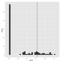
The package commands are explained in more detail in the package vignette, but the idea is simple. Running the pmc comparison between two models (for the model-choice step) looks like this:

[code lang=”R”] bm_v_lambda <- pmc(geospiza.tree, geospiza.data["wingL"],
"BM", "lambda", nboot=100)
[/code]

Extracting the distribution of estimates for the parameter lambda got from fitting the lambda model (B) to data made by simulating under lambda model (A):

[code lang=”R”] lambdas <- subset(bm_v_lambda["par_dists"],
comparison=="BB" & parameter=="lambda")
[/code]

To view the model comparison, just plot the pmc result:

[code lang=”R”]plot(bm_v_lambda)[/code]

The substantial overlap in the likelihood ratios after simulating under either model indicate that we cannot choose between BM and lambda in this case. I’ll leave the paper to explain this approach in more detail, but it’s just simulation and refitting.

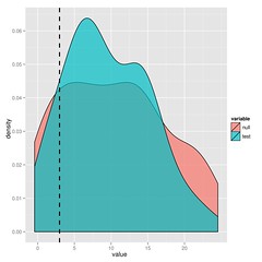
You could just bootstrap the likelihoods or for nested models, look at the parameter distributions, but you get the maximum statistical power from the ratio (says Neyman-Pearson Lemma).

A technical note: mix and match formats

Many users don’t like going between ouch format and ape/phylo formats. The pmc package doesn’t care what you use, feel free to mix and match. In case the conversion tools are useful, I’ve provided functions to move your data and trees back and forth between those formats too. See format_data() to data-frames and convert() to toggle between tree formats.

Reproducible Research

The package is designed to make things easier. It comes with a vignette (written in sweave) showing just what commands to run to replicate the results from the manuscript.

This entire project has been documented in my open lab notebook from its inception. Posts prior to October 2010 can be found on my OWW notebook, the rest in my current phylogenetics notebook (here on wordpress). Of course this project is interwoven with many notes on related and more recent work.

Additional methods and feedback

As we discuss in the paper, simulation and randomization-based methods have an established history in this field[cite]10.1371/journal.pbio.0040373[/cite], [cite]10.1111/j.1558-5646.2010.01025.x[/cite]. These are promising things to do, and we should do them more often, but I might make a few comments on these approaches.

We are not getting a real power test when we simulate data produced from different models whose parameters have been arbitrarily assigned, rather than estimated on the same data, lest we overestimate the power. Of course we need to have a likelihood function to be able to estimate those parameters, which is not always available.

It is also common and very useful to assign some summary statistic whose value is expected to be very different under different models of evolution, and look at it’s distribution under simulation. This is certainly valid and has ties to cutting edge approaches in ABC methods, but will be less statistically powerful than if we can calculate the likelihoods of the models directly and compare those, as we do here.

Showcasing the latest phylogenetic methods: AUTEUR

July 20, 2011 / pcwainwr / 4 Comments

While high-speed fish feeding videos may be the signature of the lab, dig a bit deeper and you’ll find a wealth of comparative phylogenetic methods sneaking in. It’s a natural union — expert functional morphology is the key to good comparative methods, just as phylogenies hold the key to untangling the evolutionary origins of that morphology. The lab’s own former graduate, Brian O’Meara, made a revolutionary step forward in the land of phylogenetic methods when he unveiled Brownie in 2006, allowing researchers to identify major shifts in trait diversification rates across the tree. This work spurred not only a flood of empirical applications but also methodological innovations, such as Liam’s brownie-lite, and today’s focus: Jon Eastman et al.‘s auteur package.

Auteur, short for “Accommodating uncertainty in trait evolution using R,” is the grown-up Bayesian RJMCMC version of that original idea in Brownie. Diversification rates can change along the phylogenetic tree — only this time, you don’t have to specify where those changes could have occurred, or how many there may have been — auteur simply tries them all.

If you want the details, definitely go read the paper — it’s all there, clear and thorough. Meanwhile, what we really want to do, is take it out for a test drive.

The package isn’t up on CRAN yet, so you can grab the development version from Jon’s github page, or click here. Put that package in a working directory and fire up R in that directory. Let’s go for a spin.

[sourcecode language=”R”] install.packages("auteur_0.11.0612.tar.gz", repos=NULL)
library(auteur)

[/sourcecode]

Great, the package installed and loaded successfully. Looks like Jon’s put all 73 functions into the NAMESPACE, but it’s not hard to guess which one looks like the right one to start with. rjmcmc.bm. Yeah, that looks good. It has a nice help file, with — praise the fish — example code. Looks like we’re gonna run a simulation, where we know the answer, and see how it does:

[sourcecode language=”R”]

#############
## generate tree
n=24
while(1) {
phy=prunelastsplit(birthdeath.tree(b=1,d=0,taxa.stop=n+1))
phy$tip.label=paste("sp",1:n,sep="")
rphy=reorder(phy,"pruningwise")

# find an internal edge
anc=get.desc.of.node(Ntip(phy)+1,phy)
branches=phy$edge[,2] branches=branches[branches>Ntip(phy) & branches!=anc] branch=branches[sample(1:length(branches),1)] desc=get.descendants.of.node(branch,phy)
if(length(desc)>=4) break()
}
rphy=phy
rphy$edge.length[match(desc,phy$edge[,2])]=phy$edge.length[match(desc,phy$edge[,2])]*64

e=numeric(nrow(phy$edge))
e[match(c(branch,desc),phy$edge[,2])]=1
cols=c("red","gray")
dev.new()
plot(phy,edge.col=ifelse(e==1,cols[1],cols[2]), edge.width=2)
mtext("expected pattern of rates")

#############
## simulate data on the ‘rate-shifted’ tree
dat=rTraitCont(phy=rphy, model="BM", sigma=sqrt(0.1))

[/sourcecode]

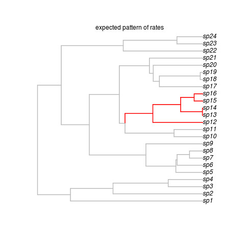
That creates this beautiful example (sorry, no random generator seed, you’re results may vary but that’s ok) tree:

Okay, so that’s the target, showing where the shift occurred. Note the last line got us some data on this tree. We’re ready to run the software. It looks super easy:

[sourcecode language=”R”] ## run two short reversible-jump Markov chains
r=paste(sample(letters,9,replace=TRUE),collapse="")
lapply(1:2, function(x) rjmcmc.bm(phy=phy, dat=dat, ngen=10000, sample.freq=10, prob.mergesplit=0.1, simplestart=TRUE, prop.width=1, fileBase=paste(r,x,sep=".")))
[/sourcecode]

The data is going in as “phy” and “dat”, just as expected. We won’t worry about the optional parameters that follow for the moment. Note that because we use lapply to run multiple chains, it would be super easy to run this on multiple processors.

Note that Jon’s creating a bunch of directories to store parameters, etc. This can be important for MCMC methods where chains get too cumbersome to handle in memory. Enough technical rambling, let’s merge and load those files in now, and plot what we got:

[sourcecode language=”R”] # collect directories
dirs=dir("./",pattern=paste("BM",r,sep="."))
pool.rjmcmcsamples(base.dirs=dirs, lab=r)

## view contents of .rda
load(paste(paste(r,"combined.rjmcmc",sep="."),paste(r,"posteriorsamples.rda",sep="."),sep="/"))
print(head(posteriorsamples$rates))
print(head(posteriorsamples$rate.shifts))

## plot Markov sampled rates
dev.new()
shifts.plot(phy=phy, base.dir=paste(r,"combined.rjmcmc",sep="."), burnin=0.5, legend=TRUE, edge.width=2)

# clean-up: unlink those directories
unlink(dir(pattern=paste(r)),recursive=TRUE)
[/sourcecode]

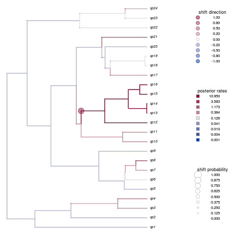
Not only is that a beautiful plot, but it’s nailed the shift in species 12-16. How’d your example do?

Auteur comes with three beautiful large data sets described in the paper. Check them out, but expect longer run times than our simple example!

[sourcecode language=”R”]

data(chelonia)
# take a look at this data
> chelonia
$phy
Phylogenetic tree with 226 tips and 225 internal nodes.

Tip labels:
Elseya_latisternum, Chelodina_longicollis, Phrynops_gibbus, Acanthochelys_radiolata, Acanthochelys_macrocephala, Acanthochelys_pallidipectoris, …

Rooted; includes branch lengths.

$dat
Pelomedusa_subrufa Pelusios_williamsi
2.995732 3.218876
…
dat <- chelonia$dat
phy <- chelonia$phy
## ready to run as above

[/sourcecode]

Thanks Jon and the rest of the Harmon Lab for a fantastic package. This is really just a tip of the iceberg, but should help get you started. See the paper for a good example of posterior analyses requisite after running any kind of MCMC, or stay tuned for a later post.

Explosive evolution in pupfish

May 5, 2011 / pcwainwr / 1 Comment

Pupfish are indeed the only group of fish named after puppy dogs for their playful behavior. They’re best known for their ability to survive in extreme environments, like desert hot springs. However, for my dissertation research, I have focused on understanding their evolution and diversification.

Pupfish show a remarkable pattern of adaptive diversification: in only two small lake systems throughout their entire range, pupfishes are evolving from 50 – 130 times faster than all other pupfish species. Truly ‘explosive evolution‘ – the fastest morphological diversification rates measured so far in fishes, and one of the fastest rates documented among all organisms. Further, other pupfish groups of similar young age do not show such extreme rates.

Figure 3 in paper. The pupfish heat map. Colors indicate the rate of evolution for 16 traits relative to other pupfishes in a: Lake Chichancanab pupfishes and b: San Salvador Island pupfishes.

What is going on here? The short answer is the evolution of novel ecological niches. Cyprinodon pupfishes occur throughout the Caribbean and along the Atlantic coast from Massachusetts to Venezuela and as far inland as isolated springs in California and Mexico. Throughout their entire range, pupfishes are ecological generalists: they eat mostly algae, decaying vegetation, and whatever insects or crustaceans they can catch. Yumm! Although different species can often be distinguished by differences in male coloration, or subtle differences in body or fin shape, pupfish species on the whole are anatomically very similar, particularly in jaw shape. Further, multiple pupfish species never coexist in the same habitat.

Except in two places. These are the only two places throughout their entire range where multiple pupfish species coexist and specialize on entirely new resources. On the tiny island of San Salvador in the Bahamas (only 11 miles long!), three pupfish species coexist in the inland salty lakes. Incredibly, one of these has evolved to feed almost entirely on the scales of other pupfishes! While scale-eating has evolved at least 14 times in other groups of fishes, within the 1,500 species of atherinimorphs, to which pupfish belong, this undescribed pupfish species is the only known scale-eater! While previous researchers speculated that it may eat scales or other fish, I was stunned to find only scales and no whole fish when I began examining the guts of this species (n = 60). This behavior is easy to watch in the field – the scale-eater stalks any nearby pupfish, quickly orienting perpendicular to its prey, striking and biting off scales, then stealthily moving on to the next target, just like a pup-tiger.

Cyprinodon sp. ‘scale-eater’: Males in full breeding coloration photographed in their natural habitat on San Salvador Island.

There is a second ecologically specialized species in these San Salvador lakes. This species has shortened jaws for crushing its diet of snails and ostracods. Moreover, it has a nose! This is one of the few fish species that tucks its jaw underneath protruding nasal tissue surrounding protruding bones (maxilla and nasal) on the face of the fish.

Cyprinodon sp. ‘nose’ What looks like an upper lip in this photo is actually the fish’s nose protruding outward above the fish’s tucked upper jaw.

The function of this peculiar fish nose is so far unknown (or any fish nose, for that matter). I do have a couple guesses: perhaps it helps stabilize the fish’s jaw while crushing hard shells. Or, it may help with species recognition, as males gently nudge females when trying to entice them to spawn.

The second remarkable place for pupfish diversification is Lake Chichancanab, Mexico, a large, brackish lake in the center of the Yucatan peninsula (Chichancanab is Mayan for “little lake” or “little girl lake”, whichever you prefer). Chichancanab contained at least five coexisting species of pupfishes, including four ecological specialists. One of these, Cyprinodon maya, is the largest pupfish species known and also the only pupfish to eat other fish. A second species, Cyprinodon simus, is the second smallest pupfish species, and was observed feeding on zooplankton in large shoals in open water. Piscivory and zooplanktivory are unique pupfish niches found only in Lake Chichancanab.

Terribly, these descriptions of Chichancanab species are in past tense. In the early 1990’s, invasive African tilapia (probably Oreochromis mossambicus) were introduced to Lake Chichancanab. In addition, the native Mexican tetra, Astyanax sp., was also introduced. All specialized pupfish species promptly declined in abundance and frequency over the next 10 years. I visited the lake in 2009 and after surveying thousands and thousands of fish from several different basins of the large lake, I observed zero Cyprinodon maya and only one putative hybrid Cyprinodon simus. These specialized species are now functionally extinct in the lake. Thankfully, they have survived in home aquaria and backyard fish ponds in the US thanks to the efforts of dedicated aquarium hobbyists in the American Killifish Association. I am now maintaining these extinct-in-the-wild species in the lab as well.

Cleared and stained specimenof Cyprinodon maya (top), the only piscivore pupfish.

Cleared and stained specimen of Cyprinodon simus (bottom), the only zooplanktivore pupfish. Note the dramatic difference in the thickness of their lower and upper jaws. These specimens were collected in the wild before invasive species were introduced and generously loaned for this research by the University of Michigan Museum of Zoology.

Thus, in only two remarkable lake systems throughout their entire range, pupfish are speciating and adapting to novel trophic resources, like scales, snails, other fish, and plankton. These two groups of pupfishes also happen to be showing the fastest rates of evolution among all pupfishes. Probably not a coincidence: invasion of these novel ecological niches is driving incredible rates of morphological change, particularly in jaw shape.

It is particularly remarkable to see this pattern within pupfish, a group of fishes that has repeatedly been isolated in new, extreme environments and also probably has repeatedly adapted to these new environments. Several other groups of pupfishes were also evolving fast in my analysis – around 5 – 10 times faster than average, such as the groups containing the Devil’s Hole pupfish, a tiny species restricted to the smallest habitat of any known organism, a tiny cave shaft in Death Valley, shown here:

Devil’s Hole, Death Valley National Park, Nevada. This vertical shaft of water stays a balmy 94 degrees F year-round and divers have not yet found the bottom (at least 400 feet deep). Cyprinodon diabolis is restricted to eating scarce algae off a tiny rock shelf near the surface and its population size has fluctuated between 37 and around 400 fish.

Cyprinodon pachycephalus also belongs to a quickly evolving group. This is the pupfish species that lives and breeds in the hottest waters of any known vertebrate, 114 degrees Fahrenheit year-round!

These are incredibly extreme environments that would be expected to drive rapid rates of morphological evolution. Indeed, these species are changing quickly, but the Devil’s hole pupfish and C. pachycephalus are both generalist detritivores, just like their relatives.

However, to really see explosive evolution appears to require that pupfish start dabbling in entirely new ways of life, to go where no pupfish has ever gone before. (this wouldn’t be blogging without Star Trek!)

But, I haven’t yet fully answered the question I originally posed. Why have novel trophic niches evolved in these two places and nowhere else across their entire range? Certainly, the size of these two lakes and lack of competitors (except native mosquitofishes) plays a role. But, there may be many similar lakes with similar fish communities throughout the Caribbean. What is going on here? This remains an outstanding research question, one I am actively pursuing.

For the full story and contact information, please see the paper:

Martin and Wainwright. In press. Trophic novelty is linked to extremes rates of morphological diversification in two adaptive radiations of Cyprinodon pupfishes. Evolution.

Modeling the distribution of sasquatch – the first published study using ENMTools

July 6, 2009 / pcwainwr / 0 Comments

Lozier, Aniello, and Hickerson just published a paper in the Journal of Biogeography in which they use sasquatch sightings and footprints to model the distribution of this elusive imaginary species. They went one step further and modeled the effects of climate change on sasquatch distributions, showing that our furry friends are only going to become more elusive with time. Finally, they used ENMTools to demonstrate that sasquatch distributions were statistically indistinguishable from those of the black bear, suggesting that many of the bigfoot sightings may have been a case of mistaken identity.

Just to put a punchline on the whole thing, the public response to the New Scientist article about the study has led to a rush of public comments claiming that the study is biased due to the a priori assumption that sasquatch isn’t real.

Stickleblog: Caught in the act

May 22, 2009 / pcwainwr / 0 Comments

This week, I’m going to discuss a cool paper that came out of Dolph Schluter’s lab in 2008. The paper zooms in on a particularly interesting part of stickleback evolution, the transition between an ancestral marine form that breeds in fresh water to a population that lives in freshwater year-round.

Usually, (and this is one of the “color-coded for your convenience” things that make stickleback a fantastic model system) you can get a good idea where a stickleback is from by looking at its armor plates. Stickleback from marine habitats tend to have a full complement of plates, whereas sticklebacks from freshwater habitats will have few to no plates:

Stickleback armor plate phenotypes: fully plated (top), partially plated(middle), low plated(bottom)

The authors sorted through hundreds of marine stickleback to find fish that had intermediate numbers of plates, which signified that they were heterozygotes for the gene that governs plate number, Eda. These fish were placed in experimental ponds and allowed to breed. Because the fish were heterozygotes for Eda, they produced offspring with high, medium, and low plates, which gave the authors a chance to observe if natural selection favored the low-plated form in freshwater.

In each pond, the frequency of the low allele increased over time, and in a similar way. There was a slight dip when fish were very young, but then frequency increased until the fish reached breeding condition. Interestingly, fish carrying the low allele grew faster and reached breeding condition sooner than fish carrying the high allele, probably because building armor plates takes energy that could be spent on growing more quickly.

The story is more complicated than that, though – not only is there a period early in life where the high allele appears to be favored, but there is also a point where fish with intermediate plates have the highest fitness, which is difficult to explain. The authors raise the possibility that the Eda gene that controls plates in stickleback may affect other traits (pleiotropy). Either way, it looks like even the most well-understood stickleback phenotype has more to tell us.

Barrett, R., Rogers, S., & Schluter, D. (2008). Natural Selection on a Major Armor Gene in Threespine Stickleback Science, 322 (5899), 255-257 DOI: 10.1126/science.1159978

Stickleblog: Sticklebacks (in) rock

May 15, 2009 / pcwainwr / 0 Comments

There are millions of sticklebacks across the globe, but you can also find sticklebacks in fossil form. The scientific name for most fossil sticklebacks is Gasterosteus doryssus, but morphologically this fossil “species” belongs within the threespine stickleback complex.

One Miocene fossil site has offered up some fascinating insights into the pace of evolution in threespine stickleback. Today I’ll be focusing on a paper that examines evolution in diet type in this unique stickleback “population”.

A few weeks ago, I mentioned “limnetic” and “benthic” stickleback – two different morphs of freshwater stickleback that live in different places within a lake and eat different things. Limnetic stickleback generally swim in the open areas of the lake and feed on zooplankton like calanoid copepods. Benthic stickleback stay close to the lakebed and feed on insect larva and small crustaceans like gammarids and ostracods.

In an earlier paper, it was shown that you can identify whether a stickleback is benthic or limnetic just from tiny scratches on the teeth. That technique was applied to fossil sticklebacks, with some striking results: at different periods in time, the population changed from limnetic to benthic and back again to limnetic.

Most stickleback in this lake were limnetic, which makes a lot of sense – in order for the stickleback to be preserved in anoxic sediment, the lake had to be fairly deep, which opens up a lot of potential habitat for limnetic stickleback. In addition, the substrate the sticklebacks are buried in is called diatomaceous earth – basically, millions and millions of dead diatoms, a type of phytoplankton. Lots of phytoplankton swimming around suggests there was zooplankton that ate them, which would provide a perfect source of food for limnetic stickleback.

Fossil sticklebacks (photo courtesy of Michael Bell)

So what about the point in time where the population changed from limnetic to benthic? The authors suggest that because of the speed of the change – and because there are few sticklebacks from these rocks that are halfway between benthic and limnetic – it might be the case that the limnetic sticklebacks went extinct and were replaced by a new population of invading benthic stickleback.

Still, even if we can’t say for sure whether the limnetics were replaced by benthics or whether they evolved into benthics, we can say that the benthic population evolved into a limnetic population over a few thousand years, because the pattern of tooth wear changes from the heavy markings typical of a benthic to the lighter markings typical of a limnetic.

It’s rare that we can use fossils to examine how a specific population changes over time, but because we can take our understanding of modern stickleback and apply it to the fossils, we can learn a lot about the dynamics of evolutionary change.

Purnell, M., Bell, M., Baines, D., Hart, P., & Travis, M. (2007). Correlated Evolution and Dietary Change in Fossil Stickleback Science, 317 (5846), 1887-1887 DOI: 10.1126/science.1147337

Stickleblog: The stickleback family tree, part 2

May 8, 2009 / pcwainwr / 0 Comments

Some weeks ago, I discussed a large phylogenetic study that separated sticklebacks from the seahorses and pipefishes – today I’m going to discuss a phylogenetics paper that zooms in on the relationships between different sticklebacks(and their very closest relatives).

Many of the same scientists from the earlier stickleback phylogeny were involved in this paper, though there is one new face, Yale’s Tom Near, a longtime Wainwright Lab collaborator and former CPB Postdoc.

The group sequenced the mitochondrial genomes of all nine sticklebacks and stickleback relatives, and they also sequenced 11 nuclear genes. They used both maximum-likelihood and Bayesian methods to estimate a phylogenetic tree of sticklebacks.

Here’s what they found:

The mitogenome and nuclear gene data dovetail beautifully, as do the maximum-likelihood and Bayesian methods for each dataset, so there’s every reason to feel confidant about this arrangement of species.

There are a number of interesting results here: Aulorhynchidae, the family that includes the tubesnout, turns out to be paraphyletic – perhaps the Aulorhynchidae should be folded into the family Gasterosteidae and considered proper sticklebacks?

The thing I find the most interesting is the phylogenetic position of Spinachia spinachia, an elongated stickleback similar in appearance to the tubesnout. The paper suggests that perhaps Spinachia‘s elongate form is the result of convergent evolution.

It’s also worth thinking about the geographical distribution of stickleback in the context of this phylogeny: Spinachia and Apeltes, two Atlantic Ocean-only species, are grouped together, while the most basal stickleback relatives are all found in the North Pacific.

There are some interesting future directions possible here as well. One of Tom’s specialties is using fossil data to calibrate phylogenies, so it’s likely we’ll see a phylogeny in the near future that gives us an idea of the timescales of major stickleback divergence events.

KAWAHARA, R., MIYA, M., MABUCHI, K., NEAR, T., & NISHIDA, M. (2009). Stickleback phylogenies resolved: Evidence from mitochondrial genomes and 11 nuclear genes Molecular Phylogenetics and Evolution, 50 (2), 401-404 DOI: 10.1016/j.ympev.2008.10.014

Stickleblog: Sticklebacks at work

May 1, 2009 / pcwainwr / 0 Comments

Today’s Stickleblog deals with a recent paper in the journal Nature by Luke Harmon(a contributor on the blog Dechronization – check it out!), Dolph Schluter, and a number of other folks.

The paper features the threespine stickleback species pairs, which have become a famous evolutionary model system in the last several decades. In a few British Columbia lakes, you can find not one but two different kinds of stickleback – a small slim “limnetic” form that eats zooplankton in open areas of the lake, and a large deep-bodied “benthic” form that eats small invertebrates on the lake bottom.

A lot of work has already been done on the stickleback species pairs, but Harmon and the others took things in a new direction and examined whether these two specialized sticklebacks could affect the lake environment itself — in other words, are sticklebacks ecosystem engineers?

To answer the question, the researchers set up large outdoor tanks using sediment and small invertebrates from an actual stickleback lake. Then, they added fish: one set of tanks received only the limnetic, another received only the benthic, another received both limnetic and benthic, and the last set received generalist sticklebacks from a single-species lake.

The type of sticklebacks added to the tank had an effect on the invertebrate community – if the tank had limnetic sticklebacks(or limnetic+benthic), there were far fewer calanoid copepods. There were also large differences between the generalist stickleback tanks and the species-pair tanks in primary production.

The most striking finding was that sticklebacks had an effect on the clarity of water; generalist sticklebacks had significant more transparent water than any of the other treatments, and species-pair treatments had the least clear water.

A lot more work will be required to uncover exactly how the sticklebacks are producing these effects, but it seems that the difference between one generalist stickleback and an adaptive radiation of two specialist sticklebacks can have important consequences for the habitats they live in.

Harmon, L., Matthews, B., Des Roches, S., Chase, J., Shurin, J., & Schluter, D. (2009). Evolutionary diversification in stickleback affects ecosystem functioning Nature, 458 (7242), 1167-1170 DOI: 10.1038/nature07974

Stickleblog: What happens when you put a stickleback and a trout together?

April 24, 2009 / pcwainwr / 0 Comments

One of the most striking features of marine stickleback is the row of bony armor plates that run along the side of the body. These “armor plates” are actually enlarged and ossified lateral line scales, and they’re a unique feature of threespine stickleback; other sticklebacks (and tubesnouts) just have a tiny row of lateral scales at the most.

Threespine stickleback, fully armored form
(illustration from Wikimedia Commons)

Freshwater stickleback populations will often have few to no armor plates, which has prompted biologists to look into the both the genetic basis of armor loss and the effect of natural selection on plate number.

In 1992, Canadian ecologist Tom Reimchen published a paper in Evolution that shed some light on the latter question.

Tom captured wild stickleback from a freshwater lake and then put them in an enclosure with one of their chief lake predators, the cutthroat trout. Predictably, the trout would bite the stickleback and try to eat it; whenever a bitten stickleback escaped or was spit out, Tom caught it. The first 153 fish were simply preserved, and the last 143 fish were placed in aquariums and monitored for several days to see if their injuries were fatal.

Then, Tom took a look at what sort of injuries all 296 stickleback had sustained from the trout attack. In particular, were stickleback with more armor plates injured less frequently than stickleback with fewer plates? It turned out that puncture wounds from trout teeth were significantly less common in more armored stickleback.

Top graph: plate number versus puncture wounds sustained
Bottom graph: plate number versus survival

In the second group of 143 fish that had been monitored for survival, over half of the fish died, many of whom did not survive the first 24 hours (for those wondering, Tom did have a control tanks of non-injured fish in the same room – they all survived). Fish with more plates survived significantly longer than fish with fewer plates; in addition, fish with injuries exhibited significantly lower survival.

Taken together, the results suggest that having more armor plates results in fewer injuries sustained from predators, which increases the fish’s chances of survival if it escapes being eaten.

There is one interesting caveat, though: all of these fish would still qualify as “low-plated” freshwater stickleback. Most of the plate variation involved the presence of a few additional plates closer to the head – does this mean that fully-plated marine fish get the same sort of protective benefit from having armor closer to the tail?

Reimchen, T. (1992). Injuries on Stickleback from Attacks by a Toothed Predator (Oncorhynchus) and Implications for the Evolution of Lateral Plates Evolution, 46 (4) DOI: 10.2307/2409768

Stickleblog: Spines hurt, according to predators

April 10, 2009 / pcwainwr / 0 Comments

One of the distinguishing features of sticklebacks is that instead of having pelvic and dorsal fins, they have serrated bony spines that the fish can lock into place(more on the locking in a later entry).

Why would evolution result in a lineage of fishes that has spines instead of fins? The classic explanation is that spines make sticklebacks a painful meal; predators will avoid eating sticklebacks if other food is available.

In 1956, Hoogland et al tested whether stickleback spines were an effective defense against larger fish. The paper itself is 33 pages, with multiple experiments – for today’s entry, I’m going to concentrate on only two of these.

In the first experiment, pike were presented with three different types of fish: 12 threespine sticklebacks, 12 ninespine sticklebacks, and 12 carplike fish lacking spines. At first, the pike went after sticklebacks, with decidedly ouch-inducing results:

After eating one stickleback of each type, the pike focused exclusively on the fish without spines, eating all 12 of them in 5 days. Once all of these were gone, sticklebacks started disappearing, but at a much slower pace, with ninespine stickleback eaten faster than threespines. It’s difficult to conclude anything too comprehensively from this, as the authors didn’t do much in the way of replication, but it does suggest that fish predators prefer nonspined prey.

Then, the authors tried the obvious experiment – if threespine stickleback have spines that make it difficult for predators to eat them, what happens if the spines are removed? Once the spines were removed from a stickleback, predators stopped spitting them out and treated them similarly to the carplike fish.

Provided one is willing to overlook the paper’s archaic methodology and lack of rigorous statistical methods(and it is from the 1950s, remember), spines appear to decrease the deliciousness of stickleback.

Perhaps that’s why sticklebacks have never really taken off as a cuisine…

R. Hoogland, D. Morris and N. Tinbergen (1956). The Spines of Sticklebacks (Gasterosteus and Pygosteus) as Means of Defence against Predators (Perca and Esox) Behaviour, 10 (3), 205-236 DOI: 10.2307/4532857