My treebase package is now up on the CRAN repository. (Source code is up, the binaries should appear soon). Here’s a few introductory examples to illustrate some of the functionality of the package. Thanks in part to new data deposition requirements at journals such as Evolution, Am Nat, and Sys Bio, and data management plan requirements from NSF, I hope the package will become increasingly useful for teaching by replicating results and for meta-analyses that can be automatically updated as the repository grows. Please contact me with any bugs or requests (or post in the issue tracker).
Basic tree and metadata queries
Downloading trees by different queries: by author, taxa, & study. More options are described in the help file.
[code lang=”R”]
both <- search_treebase("Ronquist or Hulesenbeck", by=c("author", "author"))
dolphins <- search_treebase(‘"Delphinus"’, by="taxon", max_trees=5)
studies <- search_treebase("2377", by="id.study")
Near <- search_treebase("Near", "author", branch_lengths=TRUE)
[/code]
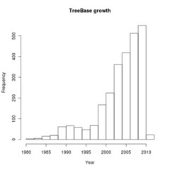
We can query the metadata record directly. For instance, plot the growth of Treebase submissions by publication date
[code lang=”R”]
all <- search_metadata("", by="all")
dates <- sapply(m, function(x) as.numeric(x$date))
hist(dates, main="TreeBase growth", xlab="Year")
[/code]
(This query could also take a date range).
How do the weekly’s do on submissions to Treebase? We construct this in a way that gives us back the indices of the matches, so we can then grab those trees directly. Run the scripts yourself to see if they’ve changed!
[code lang=”R”]
nature <- sapply(all, function(x) length(grep("Nature", x$publisher))>0)
science <- sapply(all, function(x) length(grep("^Science$", x$publisher))>0)
> sum(nature)
[1] 14
> sum(science)
[1] 14
[/code]
Now get me all of those treebase trees that have appeared in Nature.
[code lang=”R”]
s <- get_study_id( all[nature] )
nature_trees <- sapply(s, function(x) search_treebase(x, "id.study"))
[/code]
Which authors have the most submissions?
[code lang=”R”]
authors <- sapply(all, function(x){
index <- grep( "creator", names(x))
x[index]
})
a <- as.factor(unlist(authors))
> head(summary(a))
Crous, Pedro W. Wingfield, Michael J. Groenewald, Johannes Z.
88 68 58
Donoghue, Michael J. Takamatsu, Susumu Wingfield, Brenda D.
39 36 35
[/code]
Replicating results
A nice paper by Derryberry et al. appeared in Evolution recently on diversification in ovenbirds and woodcreepers [cite]10.1111/j.1558-5646.2011.01374.x[/cite]. The article mentions that the tree is on Treebase, so let’s see if we can replicate their diversification rate analysis:
Let’s grab the trees by that author and make sure we have the right one:
[code lang=”R”]
require(treebase)
search_treebase("Derryberry", "author")[[1]] -> tree
metadata(tree$S.id)
plot(tree)
[/code]
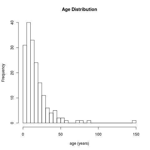
![]()
(click to zoom – go to all sizes->original size)
They fit a variety of diversification rate models avialable in the laser package, which they compare by aic.
[code lang=”R”]
require(laser)
tt <- branching.times(tree)
models <- list(pb = pureBirth(tt),
bdfit = bd(tt),
y2r = yule2rate(tt), # yule model with single shift pt
ddl = DDL(tt), # linear, diversity-dependent
ddx = DDX(tt), #exponential diversity-dendent
sv = fitSPVAR(tt), # vary speciation in time
ev = fitEXVAR(tt), # vary extinction in time
bv = fitBOTHVAR(tt)# vary both
)
aics <- sapply(models, function(x) x$aic)
# show the winning model
models[which.min(aics)]
> models[which.min(aics)]
$y2r
LH st1 r1 r2 aic
276 505.0685 1.171871 0.1426537 0.05372305 -1004.137
[/code]
Yup, their result agrees with our analysis. Using the extensive toolset for diversification rates in R, we could now rather easily check if these results hold up in newer methods such as TreePar, etc.
Meta-Analysis
Of course one of the more interesting challenges of having an automated interface is the ability to perform meta-analyses across the set of available phylogenies in treebase. As a simple proof-of-principle, let’s check all the phylogenies in treebase to see if they fit a birth-death model or yule model better.
We’ll create two simple functions to help with this analysis. While these can be provided by the treebase package, I’ve included them here to illustrate that the real flexibility comes from being able to create custom functions. ((These are primarily illustrative; I hope users and developers will create their own. In a proper analysis we would want a few additional checks.))
[code lang=”R”]
timetree <- function(tree){
check.na <- try(sum(is.na(tree$edge.length))>0)
if(is(check.na, "try-error") | check.na)
NULL
else
try( chronoMPL(multi2di(tree)) )
}
drop_errors <- function(tr){
tt <- tr[!sapply(tr, is.null)]
tt <- tt[!sapply(tt, function(x) is(x, "try-error"))]
print(paste("dropped", length(tr)-length(tt), "trees"))
tt
}
require(laser)
pick_branching_model <- function(tree){
m1 <- try(pureBirth(branching.times(tree)))
m2 <- try(bd(branching.times(tree)))
as.logical(try(m2$aic < m1$aic))
}
[/code]
Return only treebase trees that have branch lengths. This has to download every tree in treebase, so this will take a while. Good thing we don’t have to do that by hand.
[code lang=”R”]
all <- search_treebase("Consensus", "type.tree", branch_lengths=TRUE)
tt <- drop_errors(sapply(all, timetree))
is_yule <- sapply(tt, pick_branching_model)
table(is_yule)
[/code]
(cross-posted from my notebook)

Recent Comments