While high-speed fish feeding videos may be the signature of the lab, dig a bit deeper and you’ll find a wealth of comparative phylogenetic methods sneaking in. It’s a natural union — expert functional morphology is the key to good comparative methods, just as phylogenies hold the key to untangling the evolutionary origins of that morphology. The lab’s own former graduate, Brian O’Meara, made a revolutionary step forward in the land of phylogenetic methods when he unveiled Brownie in 2006, allowing researchers to identify major shifts in trait diversification rates across the tree. This work spurred not only a flood of empirical applications but also methodological innovations, such as Liam’s brownie-lite, and today’s focus: Jon Eastman et al.‘s auteur package.
Auteur, short for “Accommodating uncertainty in trait evolution using R,” is the grown-up Bayesian RJMCMC version of that original idea in Brownie. Diversification rates can change along the phylogenetic tree — only this time, you don’t have to specify where those changes could have occurred, or how many there may have been — auteur simply tries them all.
If you want the details, definitely go read the paper — it’s all there, clear and thorough. Meanwhile, what we really want to do, is take it out for a test drive.
The package isn’t up on CRAN yet, so you can grab the development version from Jon’s github page, or click here. Put that package in a working directory and fire up R in that directory. Let’s go for a spin.
[sourcecode language=”R”] install.packages("auteur_0.11.0612.tar.gz", repos=NULL)library(auteur) [/sourcecode]
Great, the package installed and loaded successfully. Looks like Jon’s put all 73 functions into the NAMESPACE, but it’s not hard to guess which one looks like the right one to start with. rjmcmc.bm. Yeah, that looks good. It has a nice help file, with — praise the fish — example code. Looks like we’re gonna run a simulation, where we know the answer, and see how it does:
[sourcecode language=”R”] #############
## generate tree
n=24
while(1) {
phy=prunelastsplit(birthdeath.tree(b=1,d=0,taxa.stop=n+1))
phy$tip.label=paste("sp",1:n,sep="")
rphy=reorder(phy,"pruningwise")
# find an internal edge
anc=get.desc.of.node(Ntip(phy)+1,phy)
branches=phy$edge[,2]
branches=branches[branches>Ntip(phy) & branches!=anc]
branch=branches[sample(1:length(branches),1)]
desc=get.descendants.of.node(branch,phy)
if(length(desc)>=4) break()
}
rphy=phy
rphy$edge.length[match(desc,phy$edge[,2])]=phy$edge.length[match(desc,phy$edge[,2])]*64
e=numeric(nrow(phy$edge))
e[match(c(branch,desc),phy$edge[,2])]=1
cols=c("red","gray")
dev.new()
plot(phy,edge.col=ifelse(e==1,cols[1],cols[2]), edge.width=2)
mtext("expected pattern of rates")
#############
## simulate data on the ‘rate-shifted’ tree
dat=rTraitCont(phy=rphy, model="BM", sigma=sqrt(0.1))
That creates this beautiful example (sorry, no random generator seed, you’re results may vary but that’s ok) tree:

Okay, so that’s the target, showing where the shift occurred. Note the last line got us some data on this tree. We’re ready to run the software. It looks super easy:
r=paste(sample(letters,9,replace=TRUE),collapse="")
lapply(1:2, function(x) rjmcmc.bm(phy=phy, dat=dat, ngen=10000, sample.freq=10, prob.mergesplit=0.1, simplestart=TRUE, prop.width=1, fileBase=paste(r,x,sep=".")))
[/sourcecode]
The data is going in as “phy” and “dat”, just as expected. We won’t worry about the optional parameters that follow for the moment. Note that because we use lapply to run multiple chains, it would be super easy to run this on multiple processors.
Note that Jon’s creating a bunch of directories to store parameters, etc. This can be important for MCMC methods where chains get too cumbersome to handle in memory. Enough technical rambling, let’s merge and load those files in now, and plot what we got:
[sourcecode language=”R”] # collect directoriesdirs=dir("./",pattern=paste("BM",r,sep="."))
pool.rjmcmcsamples(base.dirs=dirs, lab=r)
## view contents of .rda
load(paste(paste(r,"combined.rjmcmc",sep="."),paste(r,"posteriorsamples.rda",sep="."),sep="/"))
print(head(posteriorsamples$rates))
print(head(posteriorsamples$rate.shifts))
## plot Markov sampled rates
dev.new()
shifts.plot(phy=phy, base.dir=paste(r,"combined.rjmcmc",sep="."), burnin=0.5, legend=TRUE, edge.width=2)
# clean-up: unlink those directories
unlink(dir(pattern=paste(r)),recursive=TRUE)
[/sourcecode]
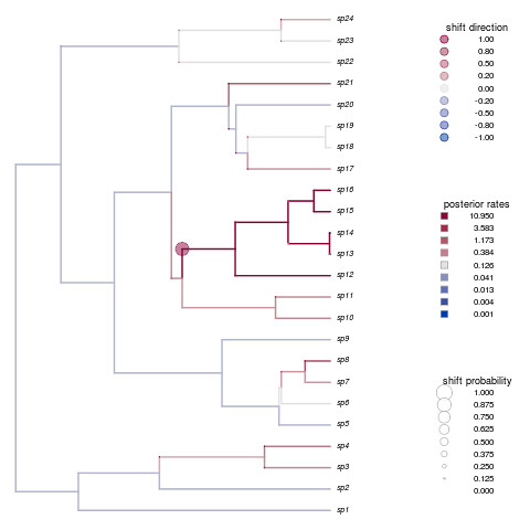
Not only is that a beautiful plot, but it’s nailed the shift in species 12-16. How’d your example do?
Auteur comes with three beautiful large data sets described in the paper. Check them out, but expect longer run times than our simple example!
[sourcecode language=”R”]data(chelonia)
# take a look at this data
> chelonia
$phy
Phylogenetic tree with 226 tips and 225 internal nodes.
Tip labels:
Elseya_latisternum, Chelodina_longicollis, Phrynops_gibbus, Acanthochelys_radiolata, Acanthochelys_macrocephala, Acanthochelys_pallidipectoris, …
Rooted; includes branch lengths.
$dat
Pelomedusa_subrufa Pelusios_williamsi
2.995732 3.218876
…
dat <- chelonia$dat
phy <- chelonia$phy
## ready to run as above
Thanks Jon and the rest of the Harmon Lab for a fantastic package. This is really just a tip of the iceberg, but should help get you started. See the paper for a good example of posterior analyses requisite after running any kind of MCMC, or stay tuned for a later post.
Recent Comments