University of California, Davis

Author: pcwainwr (Page 1 of 5)

Is your phylogeny informative?

(crossposted from my lab notebook)

Yesterday my paper [cite]10.1111/j.1558-5646.2012.01574.x[/cite] appeared in early view in Evolution,As the open access copy doesn’t appear on pubmed for a while, you can access my author’s copy here. so I’d like to take this chance to share the back-story and highlight my own view on some of our findings, and the associated package on CRAN.Just submitted, meanwhile, the code is always on github.

I didn’t set out to write this paper. I set out to write a very different paper, introducing a new phylogenetic method for continuous traits that estimates changes in evolutionary constraint. This adds even more parameters than already present in rich models multi-peak OU process, and I wanted to know if it could be justified — if there really was enough information to play the game we already had, before I went and made the situation even worse. Trying to find something rigorous enough to hang my hat on, I ended up writing this paper.

The short of it

There’s essentially three conclusions I draw from the paper.

  1. AIC is not a reliable way to select models.
  2. Certain parameters, such as \(\lambda\), a measure of “phylogenetic signal,” [cite]10.1038/44766[/cite] are going to be really hard to estimate.
  3. BUT as long as we simulate extensively to test model choice and parameter uncertainty, we won’t be misled by either of these. So it’s okay to drink the koolaid [cite]10.1086/660020[/cite], but drink responsibly.

A few reflections

I really have two problems with AIC and other information criteria when it comes to phylogenetic methods. One is that it’s too easy to simulate data from one model, and have the information criteria choose a ridiculously over-parameterized model instead. In one example, the wrong model has a \(\Delta\)AIC of 10 points over the correct model.

But a more basic problem is that it’s just not designed for hypothesis testing — it doesn’t care how much data you have, it doesn’t give a notion of significance. If we’re ascribing biological meaning to different models as different hypotheses, we need want a measure of uncertainty.

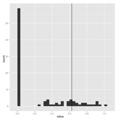
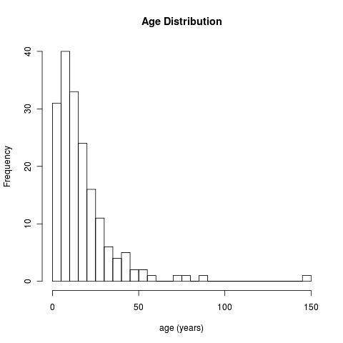
When estimating parameters that scale branch length, I think we must be cautious because these are really data-hungry, and don’t work well on small trees. Check out how few of these estimates of lambda on 100 replicate datasets hit near the correct value shown by vertical line:

The package commands are explained in more detail in the package vignette, but the idea is simple. Running the pmc comparison between two models (for the model-choice step) looks like this:

[code lang=”R”] bm_v_lambda <- pmc(geospiza.tree, geospiza.data["wingL"],
"BM", "lambda", nboot=100)
[/code]

Extracting the distribution of estimates for the parameter lambda got from fitting the lambda model (B) to data made by simulating under lambda model (A):

[code lang=”R”] lambdas <- subset(bm_v_lambda["par_dists"],
comparison=="BB" & parameter=="lambda")
[/code]

To view the model comparison, just plot the pmc result:
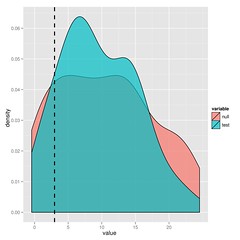
[code lang=”R”]plot(bm_v_lambda)[/code]

The substantial overlap in the likelihood ratios after simulating under either model indicate that we cannot choose between BM and lambda in this case. I’ll leave the paper to explain this approach in more detail, but it’s just simulation and refitting.

You could just bootstrap the likelihoods or for nested models, look at the parameter distributions, but you get the maximum statistical power from the ratio (says Neyman-Pearson Lemma).

A technical note: mix and match formats

Many users don’t like going between ouch format and ape/phylo formats. The pmc package doesn’t care what you use, feel free to mix and match. In case the conversion tools are useful, I’ve provided functions to move your data and trees back and forth between those formats too. See format_data() to data-frames and convert() to toggle between tree formats.

Reproducible Research

The package is designed to make things easier. It comes with a vignette (written in sweave) showing just what commands to run to replicate the results from the manuscript.

This entire project has been documented in my open lab notebook from its inception. Posts prior to October 2010 can be found on my OWW notebook, the rest in my current phylogenetics notebook (here on wordpress). Of course this project is interwoven with many notes on related and more recent work.

Additional methods and feedback

As we discuss in the paper, simulation and randomization-based methods have an established history in this field[cite]10.1371/journal.pbio.0040373[/cite], [cite]10.1111/j.1558-5646.2010.01025.x[/cite]. These are promising things to do, and we should do them more often, but I might make a few comments on these approaches.

We are not getting a real power test when we simulate data produced from different models whose parameters have been arbitrarily assigned, rather than estimated on the same data, lest we overestimate the power. Of course we need to have a likelihood function to be able to estimate those parameters, which is not always available.

It is also common and very useful to assign some summary statistic whose value is expected to be very different under different models of evolution, and look at it’s distribution under simulation. This is certainly valid and has ties to cutting edge approaches in ABC methods, but will be less statistically powerful than if we can calculate the likelihoods of the models directly and compare those, as we do here.

SICB 2012, Charleston, SC

Tomorrow some of the lab will be traveling to Charleston, South Carolina for the annual Society for Integrative and Comparative Biology meeting. Several of us are presenting on various topics including the feeding kinematics of zooplanktivores, functional morphology of sticklebacks,  nocturnality limiting diversity in the eyes of reef fish, and patterns of diversity in suction feeding among serranid fishes. Below are the times, titles and location for our talks. I’m also including the information for some previous Wainwright lab members and links to the abstracts. Hope to see you there.

Wednesday, Jan. 4  Evolutionary Morphology – Fish Feeding           08:20  Ballroom B
1.2          FULLER, P. O.*; TAKADA, T.; OUFIERO, C. E.; WAINWRIGHT, P. C.  The kinematic basis for the evolution of zooplankton feeding in haemulid fishes

Thursday, Jan. 5   Form and Function: Feeding       09:40  Ballroom C1
32.6 MCGEE, M.D.*; WAINWRIGHT, P.C.  Divergence in the functional morphology and feeding kinematics of threespine stickleback

Friday, Jan. 6      Form and Function: Underwater Light and Eyes 09:00  Room 12
76.4        SCHMITZ, Lars*; WAINWRIGHT, Peter C.  Nocturnality limits morphological and functional diversity in the eyes of reef fishes

Friday, Jan. 6      Ecomorphology: Feeding and Fighting    13:40  Ballroom C3
81.3 OUFIERO, Christopher E.*; HOLZMAN, Roi; WAINWRIGHT, Peter C.  The diversity of strike kinematics in serranid fishes: support for the ram-suction continuum

Thursday, Jan. 5   Form and Function: Feeding       09:20  Ballroom C1
32.5 COLLAR, David*; MEHTA, Rita; REVELL, Liam; ALFARO, Michael; WAINWRIGHT, Peter  Does feeding mode constrain diversification of the skull in elopomorph fishes?

Saturday, Jan. 7        Fish Feeding: Scaling and Suction   11:40  Ballroom B
94.6 HOLZMAN, R*; COLLAR, D.C.; MEHTA, R.S.; WAINWRIGHT, P.C  Suction Induced Force Field: An integrative model of aquatic feeding performance

The eyes of reef fishes

[cross-posted on my personal blog, as well]

Peter and I recently published a paper in BMC Evolutionary Biology and today the final HTML and PDF versions have become available. BMC is an open access journal, so everyone can read the paper:

Schmitz, L. & P.C. Wainwright (2011). Nocturnality constrains morphological and functional diversity in the eyes of reef fishes. BMC Evolutionary Biology, 11: 338. html, reprint.

We have several really interesting results. The eye morphology of nocturnal reef teleosts is characterized by a syndrome that indicates good light sensitivity. Nocturnal fishes have large relative eye size, high optical ratio and large, rounded pupils. However, there is a trade-off. Improved optical light sensitivity comes at the cost of reduced depth of focus and reduction of potential accommodative lens movement. Diurnal reef fishes, which are released from the stringent functional requirements of vision in dim light, have much higher morphological and optical diversity than nocturnal species. Diurnal fishes have large ranges of optical ratio, depth of focus, and lens accommodation.

This paper is the first outcome of the analysis of a data set on the eye morphology of 265 species in 43 families of teleost reef fishes. It’s an enormous amount of data. All in all, we measured 5 traits in both eyes of 849 specimens, resulting in one of the largest data sets on eye morphology ever assembled. One aspect I would like to stress is that we measured eye morphology on fresh fish (in accordance to the UC Davis animal care protocol). The fixation process that preserved specimens went through may have altered eye morphology, so we wanted to avoid this potential problem.

I also would like to highlight one of the analyses in our paper. We assessed morphological diversity of diurnal and nocturnal species by calculating the combined variance of all shape axes of a principal component analysis. However, there are far more diurnal (n=211) than nocturnal species (n=54) in the data set, and ultimately the results may be biased because of uneven sampling. Inspired by a suggestion from David Bellwood we designed a simple rarefaction analysis. We randomly re-sampled 54 diurnal species (matching the number of nocturnal species) without replacement and calculated variance on PCs 2-5, and repeated this procedure 100, 000 times. This resulted in 100,000 PC analyses with the same number of diurnal and nocturnal species, with diurnal species randomly selected anew for each run. Then, we compared the distribution of nocturnal variances to the bootstrap distribution of diurnal variances. The results are convincing and, importantly, should no longer be biased by uneven sampling. The rarefaction is easily done in ‘R’; let me know if you are interested in the code.

Finally, here are thumbnails of all figures in the paper, with links to the corresponding to the high-resolution files. Feel free to use for teaching purposes.

Live from the fish bowl

Here are some pictures of our Cal Academy team measuring fish in the project room at the California Academy of Sciences in SF. The lab has been coming here since the summer, and with the help of two undergraduates are measuring morphology on close to 250 fish species. Since there were four of us today, we needed more space and worked on display so all could see us dangling fish from sutures to get photos for center of mass estimates.

Our specimens

The team, minus one post-doc

Two post-docs hard at work

An up and coming ichthyologist

Taking lateral photos for center of mass measurements

Some new videos, the Fingered Dragonet

It’s been a while since we had a new video to post, and this will be a quick one, but it is a pretty interesting fish. We recently got some new fish in the lab, including some dragonets from the family Callionymidae. These fish are mainly found in the Indo-West Pacific in tropical waters and are typically benthic. Some from the genus Synchiropus are found in the hobby industry, but are apparently tough to maintain because they feed on benthic invertebrates. We have two species in the lab currently and have started trying to film them. One, we have had some success with, the fingered dragonet (Dactylopus dactylopus). From the videos below you can see a couple of interesting features of this fish, one is that the first two fin rays of the ventral fins are modified for walking along the bottom. This is similar to Inimicus didactylus, which you can see in a few posts back, that has the first two pectoral fins rays modified for walking. The other unique feature of this fish is the way it feeds, which is pretty different than a lot of the videos we have posted, and the topic of Sarah’s (new grad student in the Wainwright lab) dissertation. It has some pretty unique jaw protrusion!

R-TreeBASE Tutorial

My treebase package is now up on the CRAN repository. (Source code is up, the binaries should appear soon). Here’s a few introductory examples to illustrate some of the functionality of the package. Thanks in part to new data deposition requirements at journals such as Evolution, Am Nat, and Sys Bio, and data management plan requirements from NSF, I hope the package will become increasingly useful for teaching by replicating results and for meta-analyses that can be automatically updated as the repository grows. Please contact me with any bugs or requests (or post in the issue tracker).

Basic tree and metadata queries

Downloading trees by different queries: by author, taxa, & study. More options are described in the help file.

[code lang=”R”] both <- search_treebase("Ronquist or Hulesenbeck", by=c("author", "author"))
dolphins <- search_treebase(‘"Delphinus"’, by="taxon", max_trees=5)
studies <- search_treebase("2377", by="id.study")
Near <- search_treebase("Near", "author", branch_lengths=TRUE)
[/code]

We can query the metadata record directly. For instance, plot the growth of Treebase submissions by publication date

[code lang=”R”] all <- search_metadata("", by="all")
dates <- sapply(m, function(x) as.numeric(x$date))
hist(dates, main="TreeBase growth", xlab="Year")
[/code]

(This query could also take a date range).

How do the weekly’s do on submissions to Treebase? We construct this in a way that gives us back the indices of the matches, so we can then grab those trees directly. Run the scripts yourself to see if they’ve changed!

[code lang=”R”] nature <- sapply(all, function(x) length(grep("Nature", x$publisher))>0)
science <- sapply(all, function(x) length(grep("^Science$", x$publisher))>0)
> sum(nature)
[1] 14
> sum(science)
[1] 14
[/code]

Now get me all of those treebase trees that have appeared in Nature.

[code lang=”R”] s <- get_study_id( all[nature] )
nature_trees <- sapply(s, function(x) search_treebase(x, "id.study"))
[/code]

Which authors have the most submissions?

[code lang=”R”] authors <- sapply(all, function(x){
index <- grep( "creator", names(x))
x[index] })
a <- as.factor(unlist(authors))
> head(summary(a))
Crous, Pedro W. Wingfield, Michael J. Groenewald, Johannes Z.
88 68 58
Donoghue, Michael J. Takamatsu, Susumu Wingfield, Brenda D.
39 36 35
[/code]

Replicating results

A nice paper by Derryberry et al. appeared in Evolution recently on diversification in ovenbirds and woodcreepers [cite]10.1111/j.1558-5646.2011.01374.x[/cite]. The article mentions that the tree is on Treebase, so let’s see if we can replicate their diversification rate analysis:

Let’s grab the trees by that author and make sure we have the right one:

[code lang=”R”] require(treebase)
search_treebase("Derryberry", "author")[[1]] -> tree
metadata(tree$S.id)
plot(tree)
[/code]

(click to zoom – go to all sizes->original size)

They fit a variety of diversification rate models avialable in the laser package, which they compare by aic.

[code lang=”R”] require(laser)
tt <- branching.times(tree)
models <- list(pb = pureBirth(tt),
bdfit = bd(tt),
y2r = yule2rate(tt), # yule model with single shift pt
ddl = DDL(tt), # linear, diversity-dependent
ddx = DDX(tt), #exponential diversity-dendent
sv = fitSPVAR(tt), # vary speciation in time
ev = fitEXVAR(tt), # vary extinction in time
bv = fitBOTHVAR(tt)# vary both
)
aics <- sapply(models, function(x) x$aic)
# show the winning model
models[which.min(aics)] > models[which.min(aics)] $y2r
LH st1 r1 r2 aic
276 505.0685 1.171871 0.1426537 0.05372305 -1004.137
[/code]

Yup, their result agrees with our analysis. Using the extensive toolset for diversification rates in R, we could now rather easily check if these results hold up in newer methods such as TreePar, etc.

Meta-Analysis

Of course one of the more interesting challenges of having an automated interface is the ability to perform meta-analyses across the set of available phylogenies in treebase. As a simple proof-of-principle, let’s check all the phylogenies in treebase to see if they fit a birth-death model or yule model better.

We’ll create two simple functions to help with this analysis. While these can be provided by the treebase package, I’ve included them here to illustrate that the real flexibility comes from being able to create custom functions. ((These are primarily illustrative; I hope users and developers will create their own. In a proper analysis we would want a few additional checks.))

[code lang=”R”] timetree <- function(tree){
check.na <- try(sum(is.na(tree$edge.length))>0)
if(is(check.na, "try-error") | check.na)
NULL
else
try( chronoMPL(multi2di(tree)) )
}
drop_errors <- function(tr){
tt <- tr[!sapply(tr, is.null)] tt <- tt[!sapply(tt, function(x) is(x, "try-error"))] print(paste("dropped", length(tr)-length(tt), "trees"))
tt
}
require(laser)
pick_branching_model <- function(tree){
m1 <- try(pureBirth(branching.times(tree)))
m2 <- try(bd(branching.times(tree)))
as.logical(try(m2$aic < m1$aic))
}
[/code]

Return only treebase trees that have branch lengths. This has to download every tree in treebase, so this will take a while. Good thing we don’t have to do that by hand.

[code lang=”R”] all <- search_treebase("Consensus", "type.tree", branch_lengths=TRUE)
tt <- drop_errors(sapply(all, timetree))
is_yule <- sapply(tt, pick_branching_model)
table(is_yule)
[/code]

(cross-posted from my notebook)

Red lionfish: stunning and invasive

This week’s blog focuses on one of the most well recognized marine fish. Not Nemo, but the lionfish, specifically the red lionfish (Pterois volitans). Lionfish belong to the Scorpaenidae family, which includes rockfishes and Scorpionfishes. This particular species is native to the Indo-Pacific, where they can be found in lagoons and reefs in waters up to 50 meters in depth. They feed mostly on other fishes, shrimps and some crabs. One unique feature of these fish is their large pectoral fins. You can see in the video below how the pectoral fins are splayed out perpendicular to the body when initiating a strike. According to fishbase, they use these fins to trap prey in a corner, stun it and swallow it, with the aid of suction. Like most Scorpaenidae, red lionfish are venomous at the dorsal spines. However, despite this they are a common species found in home aquariums.

One thing that I was not aware of until recently about this particular species of lionfish is its invasiveness. Although red lionfish are native to the Indo-Pacific oceans, they were first documented in the Atlantic Ocean in 2000 off the coast of North Carolina, although there were some earlier reports of them off the coast of Florida in the 1990’s. The cause of invasion is most likely through the aquarium industry, whether accidental or not. While some juvenile red lionfish may make their way up to the New York area due to the Gulf Stream, their range in the Atlantic seems to extend to Cape Hatteras, North Carolina, with cold temperatures limiting further range expansion. For instance, laboratory experiments have shown they do not feed below 16C. Despite this northern limitation on their range expansion, their numbers seem to be increasing off the southeast coast of the US and into the Bahamas. In fact, they seem to be the first invasive marine species to become established off the coast of Florida. Much research has been conducted on this recent invasion, with reports documenting their effect on the recruitment of native species, and their feeding ecology in the new habitat, which seems to be primarily fishes.

The recent invasion of red lionfish to the Atlantic Ocean is just one of many examples of non-ntaive species becoming established in a new habitat and affecting the ecosystem. Florida alone has seen the establishment of several freshwater, brackish water and terrestrial species (such as pythons in the Everglades). This recent invasion has already spawned new research and will most likely provide years of research to understand the ecology of invasive species.  Who knows maybe a comparison of feeding kinematics will be done to determine the evolution of suction feeding in response to varying ecology.

This is cross-posted with my personal blog.

Steps towards understanding comparative methods

Using phylogenetic comparative methods warrants a basic understanding of the history and progress of this field.  Working with some of the more recent tools for comparative evolutionary biology, I feel compelled to find out how current methods were devised, whom to credit for the methods I use, and what assumptions I am making by using them.  Below is a list of some of the landmark papers in comparative methods, with comments and synopses (written by me and Tomomi).

Felsenstein (1981) describes the basics for creating a maximum likelihood tree from a set of nucleotide sequences. One step elaborated from his 1973 paper is Felsenstein’s pruning algorithm for calculating the likelihood of a phylogenetic tree given branch lengths and tip values.  This algorithm makes likelihood calculations more computationally efficient by eliminating redundant calculations.  The paper also describes the Markov process for finding the maximum likelihood tree from nucleotide data.  Felsenstein uses a substitution model for molecular phylogenetics in which each nucleotide has a different stationary frequency (A, C, G, and T are not expected to be equally represented at any given site on DNA sequences).  Methods for searching tree space have been improved, and Bayesian theory has since permeated phylogenetic analyses, but the pruning algorithm continues to be an important subroutine in phylogenetic computations.

Possibly the most cited paper in phylogenetic comparative methods, Felsenstein (1985) describes with clear examples why species trait values may not be statistically independent and what might be done to compensate.  Felsenstein elaborates on his method of calculating standardized contrasts (phylogenetically independent contrasts) to help overcome the non-independence of character traits.  These contrasts are basically the differences between trait values of species pairs weighted by the evolutionary change separating them; they are estimates of the rate of change over time. A common use of standardized contrasts is to look for correlation in this rate between two traits; if standardized contrasts of traits X and Y are compared in a regression analysis, a linear trend suggests correlated rates of evolution between the traits.

Schluter et al. (1997) discuss the need for error estimates on ancestral state reconstructions. The paper introduces maximum likelihood ancestral state reconstructions of both discrete and continuous characters.   Responding to Schluter et al.’s call to account for error in tree construction, Huelsenbeck et al. (2003) describe a Bayesian method for mapping the change in character states onto a phylogeny.  The introduction reiterates the importance of having an alternative to parsimony methods when tackling character change; as with maximum likelihood, the new methods allow for more than one change along a given branch in the tree.  While the Huelsenbeck et al. paper is a landmark for evolutionary analysis, it also contains a very coherent introduction to the instantaneous rate matrix, substitution model, and likelihood calculations for finding the probabilities of evolutionary histories.

Although Brownian motion is often used to model quantitative character evolution, the Ornstein-Uhlenbeck (OU) process can also be used to develop informative evolutionary models.  OU models incorporate selection as a selective optima, or adaptive peak.  OU and Brownian motion are not entirely unrelated as OU collapses to Brownian motion in the absence of selection.  Butler and King (2004) use OU to test which of several evolutionary models has the best fit to several example data sets involving anoles.  They use likelihood ratio tests to determine how various OU-based models perform against Brownian motion, observing that biological information is important in determining what models to consider.  They also stress that stasis, although positive support for stabilizing selection, is often disregarded and can lead to underestimation of evolutionary drift.  However, although they state that Brownian motion is a pure drift process, Brownian motion can provide a good fit to selective schemes under fluctuating directional selection (O’Meara et al. 2006).

While Grafen (1989) first describes a generalized least squares model for phylogenetic regressions, Chris O. from our lab pointed out the appendix of a paper on mammal intestines (Lavin et al. 2008) as a nice summary of PGLS.  This appendix describes both the history and the methods of phylogenetic regression analysis.  PGLS can be performed not only under a Brownian motion model, but also with OU and several other transformations of the variance-covariance matrix used in the mixed model approach.

These are just a handful of important papers; feel free to add to the list via comments with other references and their contributions.

By any other name

We’ve had some great posts on Fishbase and fish eyes recently, thanks to Carl and Lars. Most of the lab is working on abstracts for SICB 2012, so let’s get back to some fish videos.

This week’s contender is Petenia splendida, a fish-eating cichlid from Central America. If you saw one of this in a fish store, it would probably be called a “red bay snook”. The name isn’t particularly accurate: the fish is rarely red, doesn’t live in a bay, and isn’t a snook.

What this fish does have, though, is an impressive set of jaws for capturing prey. Petenia splendida is an impressive piscivore (fish-eater) that has some of the most protrusible jaws of any cichlid.

FishBASE from R

In lab known for its quality data collection, high-speed video style, writing the weekly blog post can be a bit of a challenge for the local code monkey. That’s right, no videos today. But lucky for me, even this group can still make good use of publicly available data. Like the other day, when one of our newer graduate students wanted to do a certain degree of data-mining from information available from FishBASE. Now I’m sure there are plenty of reasons to grumble about it, but there’s quite an impressive bit of information available on FishBASE, most of it decently referenced if by no means comprehensive. And getting that kind of information quickly and easily is rapidly becoming a skill every researcher needs. So here’s a quick tutorial of the tools to do this.

Okay, so what are we talking about? Let’s start with an example fishbase page on Nile tilapia:

Okay, so there’s a bunch of information we could start copying down, then go onto the next fish. Sounds pretty tedious for 30,000 species… Now we can get an html copy of this page, but that’s got all this messy formatting we’ll have to dispense with. Luckily, we scroll down a little farther and we see the magic words:

Download XML

The summary page takes us to just what we were looking for:

To the human eye this might not look very useful, but to a computer, it’s just what we wanted. ((Well, not acutally. A RESTful interface to this data would be better, where we could query by the different categories, finding all fish of a certain family or diet, but we’ll manage just fine from here, just might be a bit slower)) It’s XML – eXtensible Mark-up Language: meaning it’s all the stuff on the previous page, marked up with all these helpful tags so that a computer can make sense of the document. ((Actually, not everything on the html page. Between the broken links, there’s tons of information like the life history tool, diet data references, etc that somehow haven’t made it into the XML summary sheet.))

To process this, we’ll fire up our favorite language and start scripting. To access the internet from R we’ll use a the command-line url browser, curl, available in the RCurl package. We’ll process XML with the XML package, so let’s load that too. Install these from CRAN if you don’t have them:

[source lang=”r”] require(XML)
require(RCurl)
[/source]

Click on that XML link to the summary page, and note how the url is assembled: http://fishbase.sinica.edu.tw/maintenance/FB/showXML.php?identifier=FB-2&ProviderDbase=03

The thing to note here is what followers the php?. There’s something called an identifier, which is set equal to the value FB-2. 2 is the id number of Nile tilapia. Change that to 3 (leave the rest the same) and you get African perch.

We can grab the content of this page in R and parse the XML using these two packages:

[source lang=”r”] fish.id <- 2
url <- paste("http://fishbase.sinica.edu.tw/",
"maintenance/FB/showXML.php?identifier=FB-",
fish.id, "&ProviderDbase=03", sep="")
tt <- getURLContent(url, followlocation=TRUE)
doc <- xmlParse(tt)
[/source]

We create the url with a given fish id. Then the getURLContent line is the equivalent of pointing your browser to that url. Because the page is XML, we then read or parse the page with xmlParse, creating an R object representation of all that XML. We are ready to rock and roll.

If you look closely at the XML, you’ll see all these placed around the information we want, like the scientific names, identifying what they are. For instance, we see the lines that look like this:

[xml] <dwc:Family>Cichlidae</dwc:Family>
<dwc:Genus>Oreochromis</dwc:Genus>
[/xml]

Clearly these are telling us the family and the Genus for this creature. The computer just has to look for the tag (this whole entry is called a node) and that’s the family. The dwc stands for Darwin Core, which is a big language or ontology created explicitly for taxonomic applications. It tells the computer that “Family” in Darwin-Core speak, is precisely the taxonomic meaning of the word. The computer can go and look up the dwc “namespace” given at the beginning of this document to learn exactly what that word means.

To grab this text using R, we simply ask for the value of the node named dwc:Family:

[source lang=”r”] Family <- xmlValue(getNodeSet(doc, "//dwc:Family")[[1]])
Family
[/source]

There’s two commands combined in that line. getNodeSet() is the first, getting any nodes that have the name dwc:Family anywhere (the // means anywhere) in the document. The [[1]] indicates that we want the first node it finds (since there’s only one of these in the entire document). Specifying which node we want makes use of the xpath syntax, a powerful way of navigating XML which we’ll use more later.

The xmlValue command just extracts the contents of that node, now that we’ve found it. If we ask R for the value it got for Family, it says Cichlidae, just as expected.

That was easy. We can do the same for Genus, Scientific Name, etc. As we go down the XML document, we see some of the information we want isn’t given a uniquely labeled node.
For instance, the information for size, habitat, and distribution are all under nodes called . Closer look shows these nodes are under “parent” nodes, all called . If we look at the other “child” nodes of these nodes, we see they also have a node called , like this:

[xml] <dataObject>
<dc:identifier>FB-Size-2</dc:identifier>
… other stuff ….
<dc:description> Text We need </dc:description>
… other stuff ….
</dataObject>
[/xml]

That identifier node tells us that this dataObject has size information. We can grab the content of that dc:description by first finding the identifier that says FB-Size-2, going up to it’s parent dataObject, and asking that dataObject for it’s child node called description. Like this:

[source lang=”r”] size_node <- getNodeSet(doc, paste("//dc:identifier[string(.) =
FB-Size-", fish.id, "’]/..", sep=""))
size <- xmlValue( size_node[[1]][["description"]] )
[/source]

Okay, so that looks crazy complicated — guess we got in a bit deep. See that link to xpath above? That’s a wee tutorial that will explain most of what’s going on here. It’s pretty simple if you take it slow. Using these kind of tricks, we can extract just the information we need from the XML.

Meanwhile, if you want the fast-track option, I’ve put this together in a little R package called rfishbase. The package has a function called fishbase() which extracts various bits of information using these calls. Once you get the hang of it you can modify it pretty easily. I do a little extra processing to get numbers from text using Regular Expressions, a sorta desperate but powerful option when everything isn’t nicely labeled XML.

Using this function we query a fish id number and get back the data in a nice R list, which we can happily manipulate. Here’s a quick demo:

[source lang=”r”] require(rfishbase)

## a general function to loop over all fish ids to get data
getData <- function(fish.ids){
suppressWarnings(
lapply(fish.ids, function(i) try(fishbase(i)))
)
}

# A function to extract the ages, handling missing values
get.ages <- function(fish.data){
sapply(fish.data, function(out){
if(!(is(out,"try-error")))
x <- out$size_values[["age"]] else
x <- NA
x
})

}

# Process all the XML first, then extract the ages
fish.data <- getData(2:500)
yr <- get.ages(fish.data)

# Plot data
hist(yr, breaks=40, main="Age Distribution", xlab="age (years)");
[/source]

Note we take a bit of care to avoid the missing values using try() function. Here’s the results:

Kinda cool, isn’t it?

« Older posts

© 2024 Wainwright Lab

Theme by Anders NorenUp ↑