University of California, Davis

Category: software

FishBASE from R

In lab known for its quality data collection, high-speed video style, writing the weekly blog post can be a bit of a challenge for the local code monkey. That’s right, no videos today. But lucky for me, even this group can still make good use of publicly available data. Like the other day, when one of our newer graduate students wanted to do a certain degree of data-mining from information available from FishBASE. Now I’m sure there are plenty of reasons to grumble about it, but there’s quite an impressive bit of information available on FishBASE, most of it decently referenced if by no means comprehensive. And getting that kind of information quickly and easily is rapidly becoming a skill every researcher needs. So here’s a quick tutorial of the tools to do this.

Okay, so what are we talking about? Let’s start with an example fishbase page on Nile tilapia:

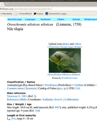
Okay, so there’s a bunch of information we could start copying down, then go onto the next fish. Sounds pretty tedious for 30,000 species… Now we can get an html copy of this page, but that’s got all this messy formatting we’ll have to dispense with. Luckily, we scroll down a little farther and we see the magic words:

Download XML

The summary page takes us to just what we were looking for:

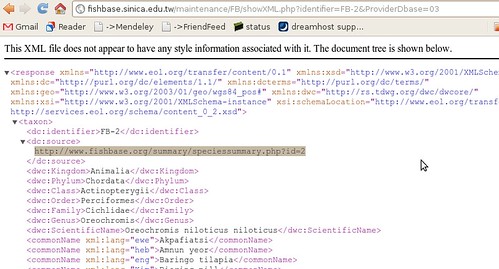
To the human eye this might not look very useful, but to a computer, it’s just what we wanted. ((Well, not acutally. A RESTful interface to this data would be better, where we could query by the different categories, finding all fish of a certain family or diet, but we’ll manage just fine from here, just might be a bit slower)) It’s XML – eXtensible Mark-up Language: meaning it’s all the stuff on the previous page, marked up with all these helpful tags so that a computer can make sense of the document. ((Actually, not everything on the html page. Between the broken links, there’s tons of information like the life history tool, diet data references, etc that somehow haven’t made it into the XML summary sheet.))

To process this, we’ll fire up our favorite language and start scripting. To access the internet from R we’ll use a the command-line url browser, curl, available in the RCurl package. We’ll process XML with the XML package, so let’s load that too. Install these from CRAN if you don’t have them:

[source lang=”r”] require(XML)
require(RCurl)
[/source]

Click on that XML link to the summary page, and note how the url is assembled: http://fishbase.sinica.edu.tw/maintenance/FB/showXML.php?identifier=FB-2&ProviderDbase=03

The thing to note here is what followers the php?. There’s something called an identifier, which is set equal to the value FB-2. 2 is the id number of Nile tilapia. Change that to 3 (leave the rest the same) and you get African perch.

We can grab the content of this page in R and parse the XML using these two packages:

[source lang=”r”] fish.id <- 2
url <- paste("http://fishbase.sinica.edu.tw/",
"maintenance/FB/showXML.php?identifier=FB-",
fish.id, "&ProviderDbase=03", sep="")
tt <- getURLContent(url, followlocation=TRUE)
doc <- xmlParse(tt)
[/source]

We create the url with a given fish id. Then the getURLContent line is the equivalent of pointing your browser to that url. Because the page is XML, we then read or parse the page with xmlParse, creating an R object representation of all that XML. We are ready to rock and roll.

If you look closely at the XML, you’ll see all these placed around the information we want, like the scientific names, identifying what they are. For instance, we see the lines that look like this:

[xml] <dwc:Family>Cichlidae</dwc:Family>
<dwc:Genus>Oreochromis</dwc:Genus>
[/xml]

Clearly these are telling us the family and the Genus for this creature. The computer just has to look for the tag (this whole entry is called a node) and that’s the family. The dwc stands for Darwin Core, which is a big language or ontology created explicitly for taxonomic applications. It tells the computer that “Family” in Darwin-Core speak, is precisely the taxonomic meaning of the word. The computer can go and look up the dwc “namespace” given at the beginning of this document to learn exactly what that word means.

To grab this text using R, we simply ask for the value of the node named dwc:Family:

[source lang=”r”] Family <- xmlValue(getNodeSet(doc, "//dwc:Family")[[1]])
Family
[/source]

There’s two commands combined in that line. getNodeSet() is the first, getting any nodes that have the name dwc:Family anywhere (the // means anywhere) in the document. The [[1]] indicates that we want the first node it finds (since there’s only one of these in the entire document). Specifying which node we want makes use of the xpath syntax, a powerful way of navigating XML which we’ll use more later.

The xmlValue command just extracts the contents of that node, now that we’ve found it. If we ask R for the value it got for Family, it says Cichlidae, just as expected.

That was easy. We can do the same for Genus, Scientific Name, etc. As we go down the XML document, we see some of the information we want isn’t given a uniquely labeled node.
For instance, the information for size, habitat, and distribution are all under nodes called . Closer look shows these nodes are under “parent” nodes, all called . If we look at the other “child” nodes of these nodes, we see they also have a node called , like this:

[xml] <dataObject>
<dc:identifier>FB-Size-2</dc:identifier>
… other stuff ….
<dc:description> Text We need </dc:description>
… other stuff ….
</dataObject>
[/xml]

That identifier node tells us that this dataObject has size information. We can grab the content of that dc:description by first finding the identifier that says FB-Size-2, going up to it’s parent dataObject, and asking that dataObject for it’s child node called description. Like this:

[source lang=”r”] size_node <- getNodeSet(doc, paste("//dc:identifier[string(.) =
FB-Size-", fish.id, "’]/..", sep=""))
size <- xmlValue( size_node[[1]][["description"]] )
[/source]

Okay, so that looks crazy complicated — guess we got in a bit deep. See that link to xpath above? That’s a wee tutorial that will explain most of what’s going on here. It’s pretty simple if you take it slow. Using these kind of tricks, we can extract just the information we need from the XML.

Meanwhile, if you want the fast-track option, I’ve put this together in a little R package called rfishbase. The package has a function called fishbase() which extracts various bits of information using these calls. Once you get the hang of it you can modify it pretty easily. I do a little extra processing to get numbers from text using Regular Expressions, a sorta desperate but powerful option when everything isn’t nicely labeled XML.

Using this function we query a fish id number and get back the data in a nice R list, which we can happily manipulate. Here’s a quick demo:

[source lang=”r”] require(rfishbase)

## a general function to loop over all fish ids to get data
getData <- function(fish.ids){
suppressWarnings(
lapply(fish.ids, function(i) try(fishbase(i)))
)
}

# A function to extract the ages, handling missing values
get.ages <- function(fish.data){
sapply(fish.data, function(out){
if(!(is(out,"try-error")))
x <- out$size_values[["age"]] else
x <- NA
x
})

}

# Process all the XML first, then extract the ages
fish.data <- getData(2:500)
yr <- get.ages(fish.data)

# Plot data
hist(yr, breaks=40, main="Age Distribution", xlab="age (years)");
[/source]

Note we take a bit of care to avoid the missing values using try() function. Here’s the results:

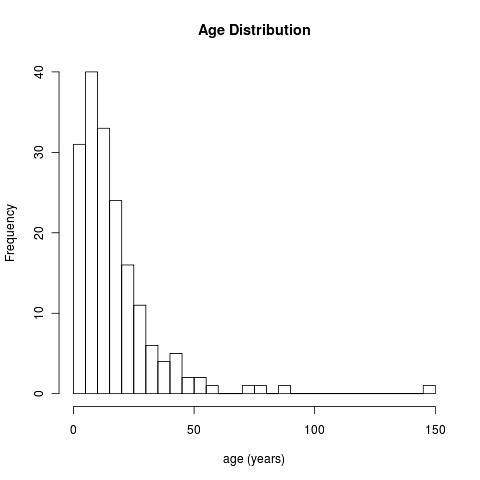
Kinda cool, isn’t it?

Showcasing the latest phylogenetic methods: AUTEUR

While high-speed fish feeding videos may be the signature of the lab, dig a bit deeper and you’ll find a wealth of comparative phylogenetic methods sneaking in.  It’s a natural union — expert functional morphology is the key to good comparative methods, just as phylogenies hold the key to untangling the evolutionary origins of that morphology.  The lab’s own former graduate, Brian O’Meara, made a revolutionary step forward in the land of phylogenetic methods when he unveiled Brownie in 2006, allowing researchers to identify major shifts in trait diversification rates across the tree.  This work spurred not only a flood of empirical applications but also methodological innovations, such as Liam’s brownie-lite, and today’s focus: Jon Eastman et al.‘s auteur package.

Auteur, short for “Accommodating uncertainty in trait evolution using R,” is the grown-up Bayesian RJMCMC version of that original idea in Brownie.  Diversification rates can change along the phylogenetic tree — only this time, you don’t have to specify where those changes could have occurred, or how many there may have been — auteur simply tries them all.

If you want the details, definitely go read the paper — it’s all there, clear and thorough.  Meanwhile, what we really want to do, is take it out for a test drive.

The package isn’t up on CRAN yet, so you can grab the development version from Jon’s github page, or click here.  Put that package in a working directory and fire up R in that directory.  Let’s go for a spin.

[sourcecode language=”R”] install.packages("auteur_0.11.0612.tar.gz", repos=NULL)
library(auteur)

[/sourcecode]

Great, the package installed and loaded successfully. Looks like Jon’s put all 73 functions into the NAMESPACE, but it’s not hard to guess which one looks like the right one to start with.  rjmcmc.bm.  Yeah, that looks good.  It has a nice help file, with — praise the fish — example code.  Looks like we’re gonna run a simulation, where we know the answer, and see how it does:

[sourcecode language=”R”]

#############
## generate tree
n=24
while(1) {
phy=prunelastsplit(birthdeath.tree(b=1,d=0,taxa.stop=n+1))
phy$tip.label=paste("sp",1:n,sep="")
rphy=reorder(phy,"pruningwise")

# find an internal edge
anc=get.desc.of.node(Ntip(phy)+1,phy)
branches=phy$edge[,2] branches=branches[branches>Ntip(phy) & branches!=anc] branch=branches[sample(1:length(branches),1)] desc=get.descendants.of.node(branch,phy)
if(length(desc)>=4) break()
}
rphy=phy
rphy$edge.length[match(desc,phy$edge[,2])]=phy$edge.length[match(desc,phy$edge[,2])]*64

e=numeric(nrow(phy$edge))
e[match(c(branch,desc),phy$edge[,2])]=1
cols=c("red","gray")
dev.new()
plot(phy,edge.col=ifelse(e==1,cols[1],cols[2]), edge.width=2)
mtext("expected pattern of rates")

#############
## simulate data on the ‘rate-shifted’ tree
dat=rTraitCont(phy=rphy, model="BM", sigma=sqrt(0.1))

[/sourcecode]

That creates this beautiful example (sorry, no random generator seed, you’re results may vary but that’s ok) tree:


Okay, so that’s the target, showing where the shift occurred.  Note the last line got us some data on this tree.  We’re ready to run the software.  It looks super easy:

[sourcecode language=”R”] ## run two short reversible-jump Markov chains
r=paste(sample(letters,9,replace=TRUE),collapse="")
lapply(1:2, function(x) rjmcmc.bm(phy=phy, dat=dat, ngen=10000, sample.freq=10, prob.mergesplit=0.1, simplestart=TRUE, prop.width=1, fileBase=paste(r,x,sep=".")))
[/sourcecode]

The data is going in as “phy” and “dat”, just as expected.  We won’t worry about the optional parameters that follow for the moment.  Note that because we use lapply to run multiple chains, it would be super easy to run this on multiple processors.

Note that Jon’s creating a bunch of directories to store parameters, etc.  This can be important for MCMC methods where chains get too cumbersome to handle in memory.  Enough technical rambling, let’s merge and load those files in now, and plot what we got:

[sourcecode language=”R”] # collect directories
dirs=dir("./",pattern=paste("BM",r,sep="."))
pool.rjmcmcsamples(base.dirs=dirs, lab=r)

## view contents of .rda
load(paste(paste(r,"combined.rjmcmc",sep="."),paste(r,"posteriorsamples.rda",sep="."),sep="/"))
print(head(posteriorsamples$rates))
print(head(posteriorsamples$rate.shifts))

## plot Markov sampled rates
dev.new()
shifts.plot(phy=phy, base.dir=paste(r,"combined.rjmcmc",sep="."), burnin=0.5, legend=TRUE, edge.width=2)

# clean-up: unlink those directories
unlink(dir(pattern=paste(r)),recursive=TRUE)
[/sourcecode]

Not only is that a beautiful plot, but it’s nailed the shift in species 12-16.  How’d your example do?

Auteur comes with three beautiful large data sets described in the paper.  Check them out, but expect longer run times than our simple example!

[sourcecode language=”R”]

data(chelonia)
# take a look at this data
> chelonia
$phy
Phylogenetic tree with 226 tips and 225 internal nodes.

Tip labels:
Elseya_latisternum, Chelodina_longicollis, Phrynops_gibbus, Acanthochelys_radiolata, Acanthochelys_macrocephala, Acanthochelys_pallidipectoris, …

Rooted; includes branch lengths.

$dat
Pelomedusa_subrufa                   Pelusios_williamsi
2.995732                             3.218876

dat <- chelonia$dat
phy <- chelonia$phy
## ready to run as above

[/sourcecode]

Thanks Jon and the rest of the Harmon Lab for a fantastic package. This is really just a tip of the iceberg, but should help get you started. See the paper for a good example of posterior analyses requisite after running any kind of MCMC, or stay tuned for a later post.

Datamuncher – a handy tool for niche and distribution modelers

Here’s a little tool I whipped together for my own use. I hope it’s useful to others as well. Basically what it does is take .csv files of species occurrences and a batch of ASCII files, and converts them into three output files. They are:

  1. A community presence/absence matrix, with “community” defined as a grid cell in the ASCII raster files.
  2. A set of coordinates for each grid cell that has at least one species present in it, corresponding to the “communities” above.
  3. A matrix of values from the ASCII raster files for each community.

The general idea is to take data in a format that is acceptable for Maxent (.csv and .asc) and convert it into a set of files that are usable with some of the R algorithms. Currently it seems to be working with GDM, but I haven’t tried anything else. You may need to delete columns 1-3 in the environment file, depending on what you’re doing with it.

Here’s the quick and dirty of it:

Where it says “occurrence files”, you just hit the “add files” button and drop in all of the .csv files you want to use. Note that everything in that box is going to be thrown into ONE set of output files!

Second, you add your environmental layers. ASCII raster format is the only one it understands.

Third, pick an output directory.

Finally, name your analysis. If your analysis is named “my_stuff”, the output files will be “my_stuff_communities.csv” (1 above), “my_stuff_community_coordinates.csv” (2), “my_stuff_environment.csv” (3), all dropped into the output directory you chose.

In addition to its original intent, this tool may also be useful to those who want a quick and dirty way to get their data extracted for a MANOVA or other analysis – if you feed it occurrence files for one species at a time, the environment file will contain all conditions occupied by that species. Neat!

You can download it as a Windows executable file here, or as a Perl script>here. Be aware that the Perl script requires that Tk be installed (NOT Tk+!), which you can do from the package manager. Also be aware that it probably won’t work on a Mac because of the way it’s parsing directories. If anyone wants a Mac version, please feel free to email me.

Also let me know if you hit any snags. Testing has been rather limited so far, as I just finished it today. Use at your own risk!

© 2024 Wainwright Lab

Theme by Anders NorenUp ↑